Loops in R

Introduction to using for loops
What Are Loops?
“Looping”, “cycling”, “iterating” or just replicating instructions is an old practice that originated well before the invention of computers. It is nothing more than automating a multi-step process by organizing sequences of actions or ‘batch’ processes and by grouping the parts that need to be repeated.
All modern programming languages provide special constructs that allow for the repetition of instructions or blocks of instructions.
Broadly speaking, there are two types of these special constructs or loops in modern programming languages. Some loops execute for a prescribed number of times, as controlled by a counter or an index, incremented at each iteration cycle. These are part of the for loop family.
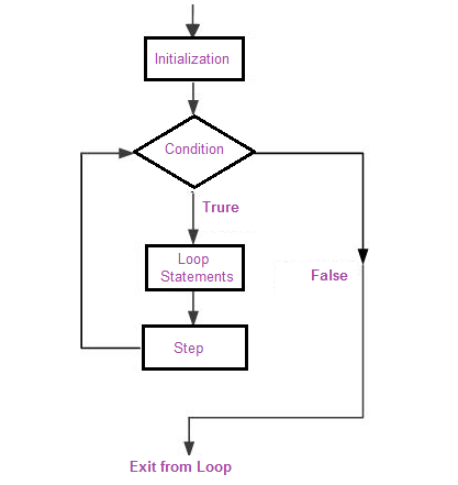
In R for loops usually are constructed as such:
for(items in list_of_items){
results <- do_something(item)

print(results)
}
Here are a few simple examples:
# Create a vector filled with random normal values
u1 <- rnorm(30)
print("This loop calculates the square of the first 10 elements of vector u1")

# Initialize `usq`
usq <- 0

for(i in 1:10) {
  # i-th element of `u1` squared into `i`-th position of `usq`
  usq[i] <- u1[i]*u1[i]
  print(usq[i])
}
[1] "This loop calculates the square of the first 10 elements of vector u1"
[1] 0.7545169
[1] 0.06958002
[1] 0.01712334
[1] 0.002240257
[1] 1.243254
[1] 0.3647912
[1] 0.1733139
[1] 3.563338
[1] 0.3366709
[1] 0.09005843
pets <- c("spot", "gigantor", "fluffy")
for (pet in pets) {
  print(pet)
}
[1] "spot"
[1] "gigantor"
[1] "fluffy"
NOTES: - notice that we include print inside a for loop in order to provide us with an output. - for loops work on many data structures (i.e. lists, vectors, arrays, matrices). - It repeats the same action until it comes to the end of the list - we can also store the outputs from a forloop into data.frames/arrays.
There are two ways we can call the sequence in the for loop. First we can actually say pick the items from the item list. But computers don’t understand names but numbers/positions. with simple for loops like the pet one above, using for (pet in pets) it is looking for a vector called pets and then sequentially going through it. We could also say for (i in 1:length(pets)) which would also work and following the sequence based on its index. There are advantages to using the latter more complicated structure when we develop for loops for complex procedures or we want to keep track of the progress of a loop (e.g. when we use Monte Carlo Simulation techniques).
Example 1: Following the stocks
now its time to work with some data. Let’s say we work in the stock exhange and want to explore and analyse trends in certain stocks. For loops can be useful with bringing in the data in an organised manner, we can plot the data and even check if any stocks have some association.
#set your working directly if need be
#setwd()
#load the libraries you need
library(tidyverse)

#make a list of the files you want to load
tech <- c("aapl", "amzn", "fb", "goog", "ibm", "msft")
#create an empty data frame to fill
dat <- data.frame()

# Read csv, add a column referring to the company
# Then combine them into one data folder
for (sym in tech) {
  filename = paste(sym, ".csv", sep="")
  t <- read.csv(filename)
  t$Symbol <- sym

  dat <- rbind(dat, t)
}
head(dat)
| Date | Open | High | Low | Close | Volume | Change | ChangePerc | Symbol |
|---|---|---|---|---|---|---|---|---|
| 2017-10-20 | 156.61 | 157.75 | 155.96 | 156.25 | 23907540 | 0.27 | 0.1728000 | aapl |
| 2017-10-19 | 156.75 | 157.08 | 155.02 | 155.98 | 42357420 | -3.78 | -2.4233876 | aapl |
| 2017-10-18 | 160.42 | 160.71 | 159.60 | 159.76 | 16252850 | -0.71 | -0.4444166 | aapl |
| 2017-10-17 | 159.78 | 160.87 | 159.23 | 160.47 | 18969700 | 0.59 | 0.3676700 | aapl |
| 2017-10-16 | 157.90 | 160.00 | 157.65 | 159.88 | 24093300 | 2.89 | 1.8076057 | aapl |
| 2017-10-13 | 156.73 | 157.28 | 156.41 | 156.99 | 16367780 | 0.99 | 0.6306134 | aapl |
# We could also write this same for loop using indexes instead
for (i in 1:length(tech)) {
  stock=tech[i]
  filename = paste(stock, ".csv", sep="")
  t <- read.csv(filename)
  t$Symbol <- stock

  dat <- rbind(dat, t)
}
head(dat)
| Date | Open | High | Low | Close | Volume | Change | ChangePerc | Symbol |
|---|---|---|---|---|---|---|---|---|
| 2017-10-20 | 156.61 | 157.75 | 155.96 | 156.25 | 23907540 | 0.27 | 0.1728000 | aapl |
| 2017-10-19 | 156.75 | 157.08 | 155.02 | 155.98 | 42357420 | -3.78 | -2.4233876 | aapl |
| 2017-10-18 | 160.42 | 160.71 | 159.60 | 159.76 | 16252850 | -0.71 | -0.4444166 | aapl |
| 2017-10-17 | 159.78 | 160.87 | 159.23 | 160.47 | 18969700 | 0.59 | 0.3676700 | aapl |
| 2017-10-16 | 157.90 | 160.00 | 157.65 | 159.88 | 24093300 | 2.89 | 1.8076057 | aapl |
| 2017-10-13 | 156.73 | 157.28 | 156.41 | 156.99 | 16367780 | 0.99 | 0.6306134 | aapl |
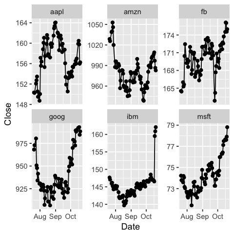
#now we can plot the data to see what each stock looks like
#used to change the size of plot
library(repr)

# Change plot size to 4 x 3
options(repr.plot.width=4, repr.plot.height=4)
#first make sure the Date variable follows the correct date structure
dat$Date <- as.Date(dat$Date)

# Now we can do facetting in ggplot!
ggplot(dat, aes(x=Date, y=Close)) +
  geom_point() +
  geom_line() +
  facet_wrap(~ Symbol, scales = "free_y")
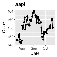
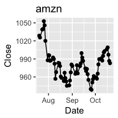
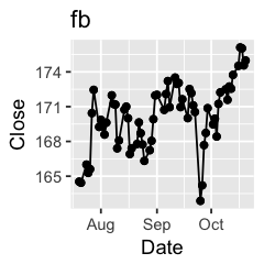
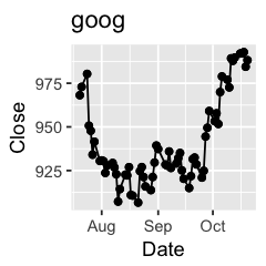
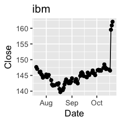
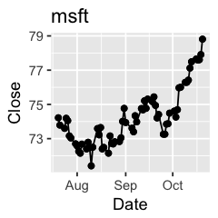
Challenge 1: Can you plot individual graphs of closing price versus time of the six companies, using for loop?
options(repr.plot.width=2, repr.plot.height=2)
for (sym in tech) {
  p <- dat %>%
    filter(Symbol == sym) %>%
    ggplot(aes(x=Date, y=Close)) +
    geom_line() +
    geom_point() +
    ggtitle(sym)
  print(p)
}
Challenge 2: Let’s say I’m interested in knowing the relationship between daily % changes in Apple’s stock price, we can use cor(X, Y) to find out the correlation. X being Apple’s % daily changes, Y being other companies’. Use a for loop to do this.
correl <- c()
X <- dat %>% filter(Symbol == "aapl") %>%
  .$ChangePerc
for (sym in tech[2:5]) {
  Y <- dat %>% filter(Symbol == sym) %>%
    .$ChangePerc
  r <- cor(X, Y, use="complete.obs") %>% round(2)
  msg <- paste("Correlation between daily changes in aapl and ", sym, " is ", r,
               ".", sep="")
  print(msg)
  correl <- c(correl, r)
}
correl
[1] "Correlation between daily changes in aapl and amzn is 0.53."
[1] "Correlation between daily changes in aapl and fb is 0.44."
[1] "Correlation between daily changes in aapl and goog is 0.43."
[1] "Correlation between daily changes in aapl and ibm is -0.07."
- 0.53
- 0.44
- 0.43
- -0.07
Example: Simulating a Markov Chain
for loops are very useful when it comes to simulations. Many researchers use markov chains in their research to simulate what a process might be doing. Markov chains is a sequence of random variables where the next value only depends on its previous value. They are used in many contexts from brownian motion in physics to stock market time series trends. The main highlight is that the process is sequential, hence for loops are used in simulating them.
Lets say we wish to simulate a Markov chain with a certain probability transition matrix and a known initial state. I.e we have three boxes and we want to move between them.
#define our transition probabilities for three states, 1. Rain, 2. Nice, 3. Snow
P <- matrix( c(0.5, 0.25, 0.5, 0.25, 0, 0.25,
               0.25, 0.5, 0.5), 3,3, byrow=TRUE)

#create a function that will simulate the markov chain by randomly sampling for a given length
simMarkov <- function( P, len=1000) {
        n <- NROW(P)
        result <- numeric(len)
        result[1] <- 1
        for (i in 2:len) {
            result[i] <- sample(1:n, 1, prob=P[ result[i-1], ])
        }
    result
 }

#now we can simulation a markov chain for a matrix of tranisiton probabilities
results <- simMarkov(P, 20)
results
- 1
- 3
- 2
- 3
- 3
- 1
- 3
- 3
- 3
- 3
- 3
- 2
- 3
- 3
- 3
- 3
- 3
- 3
- 1
- 1
Nesting for loops
For loops may be nested, but when and why would we be using this? Suppose we wish to manipulate a matrix by setting its elements to specific values; we might do something like this:
# nested for: multiplication table
mymat = matrix(nrow=10, ncol=10) # create a 10 x 10 matrix (of 10 rows and 10 columns)

for(i in 1:dim(mymat)[1])  # for each row
{
  for(j in 1:dim(mymat)[2]) # for each column
  {
    mymat[i,j] = i*j     # assign values based on position: product of two indexes
  }
}
mymat
| 1 | 2 | 3 | 4 | 5 | 6 | 7 | 8 | 9 | 10 |
| 2 | 4 | 6 | 8 | 10 | 12 | 14 | 16 | 18 | 20 |
| 3 | 6 | 9 | 12 | 15 | 18 | 21 | 24 | 27 | 30 |
| 4 | 8 | 12 | 16 | 20 | 24 | 28 | 32 | 36 | 40 |
| 5 | 10 | 15 | 20 | 25 | 30 | 35 | 40 | 45 | 50 |
| 6 | 12 | 18 | 24 | 30 | 36 | 42 | 48 | 54 | 60 |
| 7 | 14 | 21 | 28 | 35 | 42 | 49 | 56 | 63 | 70 |
| 8 | 16 | 24 | 32 | 40 | 48 | 56 | 64 | 72 | 80 |
| 9 | 18 | 27 | 36 | 45 | 54 | 63 | 72 | 81 | 90 |
| 10 | 20 | 30 | 40 | 50 | 60 | 70 | 80 | 90 | 100 |
Tips for loops
- Try to put as little code as possible within the loop by taking out as many instructions as possible (remember, anything inside the loop will be repeated several times and perhaps it is not needed).
- Careful when using repeat: ensure that a termination is explicitly set by testing a condition, or an infinite loop may occur.
- If a loop is getting (too) big, it is better to use one or more function calls within the loop; this will make the code easier to follow. But the use of a nested for loop to perform matrix or array operations is probably a sign that things are not implemented the best way for a matrix based language like R.
- Growing’ of a variable or dataset by using an assignment on every iteration is not recommended (in some languages like Matlab, a warning error is issued: you may continue but you are invited to consider alternatives). A typical example is shown in the next section.
- If you find out that a vectorization option exists, don’t use the loop as such, learn the vectorized version instead.
Vectorization
First we create an m x n matrix with replicate(m, rnorm(n)) with m=10 column vectors of n=10 elements each, constructed with rnorm(n), which creates random normal numbers. Then we transform it into a dataframe (thus 10 observations of 10 variables) and perform an algebraic operation on each element using a nested for loop: at each iteration, every element referred by the two indexes is incremented by a sinusoidal function. using a for loop in this case can be more tedious than simply using the function on the matrix:
########## a bad loop, with 'growing' data
set.seed(42);
m=10; n=10;
mymat<-replicate(m, rnorm(n)) # create matrix of normal random numbers
mydframe=data.frame(mymat)    # transform into data frame

#we can use system.stem() to check how long this takes
system.time(for (i in 1:m) {
  for (j in 1:n) {
    mydframe[i,j]<-mydframe[i,j] + 10*sin(0.75*pi)
  }
}
            )
mydframe
   user  system elapsed
      0       0       0
Here, most of the execution time consists of copying and managing the loop. Let’s see how a vectorized solution looks like:
#### vectorized version
set.seed(42);
m=10; n=10;
mymat<-replicate(m, rnorm(n))
mydframe=data.frame(mymat)
system.time(mydframe<-mydframe + 10*sin(0.75*pi))
mydframe
   user  system elapsed
      0       0       0
| X1 | X2 | X3 | X4 | X5 | X6 | X7 | X8 | X9 | X10 |
|---|---|---|---|---|---|---|---|---|---|
| 8.442026 | 8.375937 | 6.764429 | 7.526518 | 7.277066 | 7.392993 | 6.703833 | 6.027949 | 8.583775 | 8.463184 |
| 6.506370 | 9.357713 | 5.289759 | 7.775905 | 6.710011 | 6.287229 | 7.256298 | 6.980881 | 7.328989 | 6.594894 |
| 7.434196 | 5.682207 | 6.899150 | 8.106171 | 7.829231 | 8.646795 | 7.652892 | 7.694586 | 7.159508 | 7.721416 |
| 7.703930 | 6.792279 | 8.285743 | 6.462141 | 6.344363 | 7.713967 | 8.470805 | 6.117544 | 6.950171 | 8.462178 |
| 7.475336 | 6.937746 | 8.966261 | 7.576023 | 5.702787 | 7.160828 | 6.343776 | 6.528239 | 5.876739 | 5.960279 |
| 6.964943 | 7.707018 | 6.640599 | 5.354059 | 7.503886 | 7.347619 | 8.373610 | 7.652064 | 7.683065 | 6.210275 |
| 8.582590 | 6.786815 | 6.813798 | 6.286609 | 6.259675 | 7.750357 | 7.406916 | 7.839247 | 6.853928 | 5.939329 |
| 6.976409 | 4.414612 | 5.307905 | 6.220160 | 8.515169 | 7.160901 | 8.109574 | 7.534835 | 6.888311 | 5.611854 |
| 9.089492 | 4.630601 | 7.531165 | 4.656860 | 6.639622 | 4.077978 | 7.991796 | 6.185292 | 8.004414 | 7.151050 |
| 7.008354 | 8.391181 | 6.431073 | 7.107190 | 7.726716 | 7.355951 | 7.791946 | 5.971287 | 7.892841 | 7.724272 |
Alternatives to loops - the apply function
In some ocassions, you can find that for loops in R are slow. R works with data in vector form already. It is why we don’t need to say create for loops to calculate mean and instead we can use a function mean which is much faster. When we plan to conduct repetitive procedures the apply() family of functions can sometimes be faster and easier to write.
There are a variety of apply() statements that handle different use cases
lapply(): Operate across lists and vectorssapply(): Simplify output to vectormapply(): Pass multiple variables or function arguments
The functions act on an input matrix or array and apply a chosen named function with one or several optional arguments (that’s why they pertain to the so called ‘functionals’.
a simple example of apply is shown below:
# define matrix mymat by replicating the sequence 1:5 for 4 times and transforming into a matrix
mymat<-matrix(rep(seq(5), 4), ncol = 5)

# mymat sum on rows
apply(mymat, 1, sum)
## [1] 15 15 15 15
# mymat sum on columns
apply(mymat, 2, sum)
- 15
- 15
- 15
- 15
- 10
- 11
- 12
- 13
- 14