RMarkdown and bookdown
Introduction
This is an introductory post into using Bookdown. Bookdown is a powerful package that allows you to create documents embedding images, tables, and code. One great reason to use Bookdown is that you can put results and images from your code directly into your text, which reduces the chances of copying errors. For this post, I’m going to focus on creating an HTML document, though you can also create outputs in Word and PDF formats. To create PDFs, you will also need to download LaTeX. Note: throughout this document, I will be showing a code in separate boxes. To get the code to display, instead of run, the code will be commented out (with “#”). To actually run the code, you will need to remove the comment character.
Formatting text
The first part of this will discuss different text formatting. This is not an extensive list of what you can do with R Markdown and text, but it will cover the basics. The top part of the document is the YAML, which stands for Yet Another Markup Language. The YAML has a lot of the commands which control the formatting of your text. For this presentation, we’re going to keep it simple, and only include the basics. The YAML goes at the top of the document. Some items are optional, such as the title, author, and date, but output format is necessary.
YAML:
---
title: "This is my title"
author: "Name here"
date: "Today's date"
output:
  bookdown::html_document2
---
Italics
Markdown:
*words*Output:
words
Bold
Markdown:
**words**Output:
words
Bullets
Markdown:
* words
* more words
Output:
- Words
- More words
Headers
Markdown:
# Top level header
## Second level header
### Third level header
#### Fourth level header

Note: in Bookdown, you can add {-} if you don't want the header to be numbered.
Output:
Top level header
Second level header
Third level header
Fourth level header
Links
You can put links in like this:
[Link text](www.linkaddress.com)Adding Code
You can add code by putting in three backticks:
# ```
# Code goes here
# ```
You can choose different languages by defining the languages in the curly brackets
# ```{r}
# Code in R
# ```
# ```{python}
# Code in python
# ```
Muting code
Sometimes, you want to run the code without displaying it or the output. In the curly brackets, you can add in information on how you want the code to perform.
# ```{r include = FALSE}
# print("Include determines whether the code and output is put into the text or not")
# ```
Showing output without code
Other times, you may want to show the output, but without showing the code. The “echo” commands controls whether the code displays or not.
# ```{r echo = FALSE}
# print("The echo command removes the code")
# ```
## [1] "The echo command removes the code"Showing code without output
If you want to display the code without running it, you can use the “eval” command.
# ```{r eval = FALSE}
# print("The eval command determines whether you run the code.")
# ```
print("The eval command determines whether you run the code.")Removing warnings and error messages
Often, you can get warnings and messages which you don’t want to display in your documents, especially when loading packages. You can control whether these display with the “message” and “warning” commands.
# ```{r message = FALSE, warning = FALSE}
# pint("Message controls whether messages display.")
# print("Warning controls whether warnings display.")
# ```
## [1] "Message controls whether messages display."## [1] "Warning controls whether warnings display."Inline code
You can also show the code inline.
Two plus two = `#r 2+2`Two plus two = 4
Adding images
From a disk
To add an image from a disk, you have to point the code to where you want it to look
# ```{r}
#knitr::include_graphics('folder/file.jpg')
#```
From your code
But you can also add in images from your code. This is one of the most useful functions of R Markdown because any time you update the code, it will automatically update the image.
# ```{r}
# plot(mtcars$hp, mtcars$mpg)
# ```
Referencing figures
You can also caption figures and refer back to them in the text.
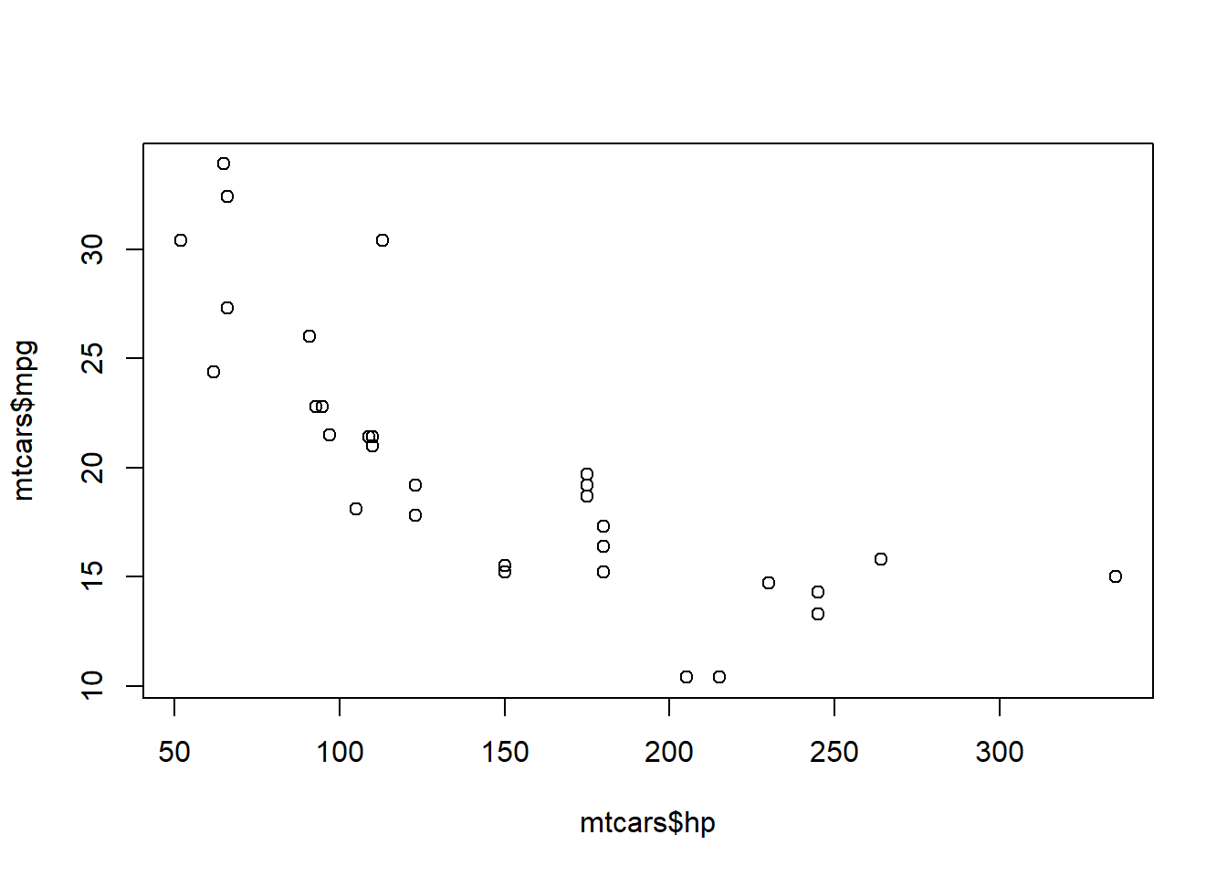
Plot the image in the code:

# ```{r hp, fig.cap= "Relationship between horsepower and miles per gallon"}
# plot(mtcars$hp, mtcars$mpg)
# ```

Then call the image in the text (Figure \@ref(fig:hp)).
Figure 1: Relationship between horsepower and miles per gallon
Then call the image in the text (Figure 1).
You can do the same for figures you call from your disk:
# ```{r horseshoe, fig.cap = "Horseshoe Bend"}
#knitr::include_graphics('folder/file.jpg')
#
#Look at this picture of Horseshoe Bend (Figure \ref@(fig:horseshoe)).
#```
Figure 2: Horseshoe Bend
Look at this picture of Horseshoe Bend (Figure 2).
Adding tables
R-markdown is not great for tables. However, there is the kable function in Knitr, which is really useful.
#```{r foo}
#install.packages("knitr")
#library(knitr)

#knitr::kable(
#  head(mtcars[,1:4]),
#  caption = "The first few rows of mtcars"
#)
#
#Check out some data in Table \@ref(tab:foo)
#```| mpg | cyl | disp | hp | |
|---|---|---|---|---|
| Mazda RX4 | 21.0 | 6 | 160 | 110 |
| Mazda RX4 Wag | 21.0 | 6 | 160 | 110 |
| Datsun 710 | 22.8 | 4 | 108 | 93 |
| Hornet 4 Drive | 21.4 | 6 | 258 | 110 |
| Hornet Sportabout | 18.7 | 8 | 360 | 175 |
| Valiant | 18.1 | 6 | 225 | 105 |
Check out some data in Table 1
Adding equations
Inline
Inline equations are denoted with the $
This is my equation: $\alpha = \beta$This is my equation: \(\alpha = \beta\)
On a separate line
If you want your equation to appear on a separate line, you can use $$
This is my equation: $$ \alpha = \beta $$This is my equation: \[\alpha = \beta\]
Referenced equations
Often, you want to number your equations so you can refer to them in the text. This takes a little bit more work but is still do-able.
\begin{equation}
\alpha = \beta
(\#eq:alpha)
\end{equation}
This is a numbered equation:
\[\begin{equation} \alpha = \beta \tag{1} \end{equation}\]Refer to Equation (1).